jupyterpidaq
User Guide
Introduction
This software allows GUI (Graphical User Interface) driven live collection, plotting and analysis of digitized data inside a Jupyter notebook using the following A-to-D interfaces:
on a Raspberry Pi:
- Adafruit compliant ADS1115 boards (example, also available from other vendors);
- The π-Plates DAQC2 plate.
on MacOS and Windows:
- Vernier LabQuest USB A-to-Ds.
demo mode on anything Jupyter runs on
- A demo mode will run on any computer with a Jupyter notebook install and Python 3.6+. Example notebooks can be found in the "usage_examples" folder.
Usage
Launch the software | Initialize data acquisiton tools | Collect data | Displaying a Data Table | Plotting data | Analyzing data
Starting JupyterPiDAQ
A working Jupyter notebook or Jupyter lab installation with JupyterPiDAQ installed is required. If you need to install the software see the Installation Instructions. There are two common ways this may be set up, that lead to slightly different steps for starting the software:
- A special kernel may be set up that can be used in any Jupyter notebook
install for the current user (see the very end of the
Installation Instructions).
- In this case launch
Jupyter, in whichever directory you want to work, using the
command:
jupyter lab(for the newer lab interface),jupyter notebook(for the modern notebook interface), orjupyter nbclassic(for the old notebook interface). - Open a new notebook and choose the kernel
for
JupyterPiDAQ. The kernel name will depend upon what was chosen during installation.
- In this case launch
Jupyter, in whichever directory you want to work, using the
command:
- Only for use within the directory structure of the virtual environment
that was set up for the software.
- In this case you must navigate to the
directory of the virtual environment using the
cdcommand before starting the software. - Then enter the virtual environment with the command
pipenv shell(you might be usingvenvor something else). This assumes you set uppipenvas described in the Installation instructions . - Launch Jupyter using the
command:
jupyter lab(for the newer lab interface),jupyter notebook(for the modern notebook interface), orjupyter nbclassic(for the old notebook interface). - Open a new python notebook.
- In this case you must navigate to the
directory of the virtual environment using the
Initialize the Data Acquisition Tools
Initialize the data acquisition tools by putting the statement from
jupyterpidaq.DAQinstance import * into the first cell and then running
(executing) the cell. The package loads supporting packages (numpy, pandas,
plotly, etc...) and searches for compatible hardware. On a Raspberry Pi this
takes a number of seconds. If no compatible A-to-D boards are found, demo
mode is used. In demo mode the A-to-D board is simulated by a random number
generator.
When setup is done a new menu appears at the end of the menubar (figure 1).
Figure 1: The menu created once the data acquisition software is initialized. Currently NOT available in Jupyter Lab.
The menu options insert jupyter widget based GUIs for starting a run, displaying the data as tables or plots, composing an expression to calculate a new column in a DataFrame, or fitting data.
Collecting data
Using the Menu
From the "DAQ Commands" menu select "Insert New run after selected cell..." This will insert the code to set up data collection for a run in the cell below the currently selected cell. Insert the name you want for the run into the code as specified. When the cell is run it will generate a GUI that looks like the figure 2, below. Fill in the information to define what you wish to do (see below figure 2 for more details).
Using a Command
In the cell you wish to collect the data enter the command
Run("desired_dataset_name"), where you replace desired_dataset_name with the
string you want for this run. Replacing spaces with _ will prevent issues,
especially on Windows. After entering the command, run the cell. This will
generate the GUI shown in figure 2.
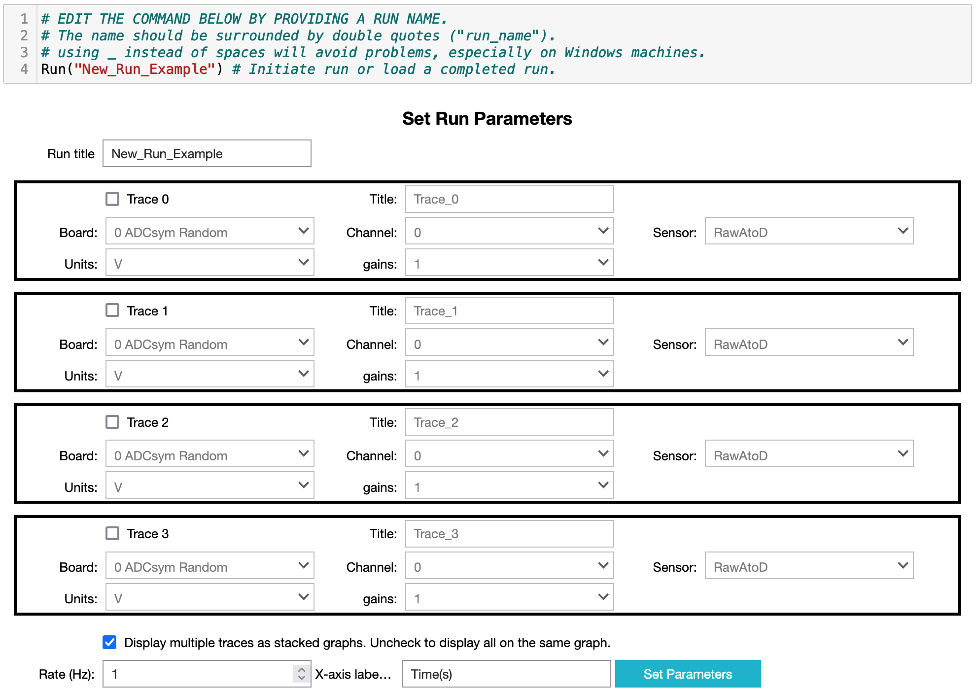
Figure 2: Image of the GUI for setting up a data collection run.
- You can give the run a different title/name using the first textbox.
- You can collect up to four (4) data traces at once. Two different data traces can display the same analog-to-digital channel, but in different units (e.g. you could record both the raw voltage and temperature from a thermistor). Each trace is activated by selecting its checkbox.
- Once a trace is activated you can give it a title and must select: the data acquisition board, channel, sensor, units and gain from the available drop-down menus.
- Once all your traces are set up decide whether they should be displayed in multiple stacked graphs or all on the same graph. Uncheck the box to display all on one graph.
- Select the data collection rate (20 Hz is currently the maximum rate, but on a Raspberry Pi you may not be able to sustain more than 5 Hz).
- When everything is set the way you wish, click on the "Set Parameters" button. The collection parameters will be displayed and a button to start the data collection will appear. You may have to scroll back up to the display as Jupyter sometimes jumps too far down when a cell is updated.
- The "start" button will convert to a "stop" button once data collection is started. The data graph(s) will update at roughly 1 Hz, so you can monitor the progress of the data collection.
- Click the "stop" button to end data collection. It can take a while to stop if the data collection has got ahead of the graphic display of the data.
- Once collection is stopped you will see a plot or plots of the completed data collection and the name of the .html file the raw data has been backed up to.
- Should you accidentally clear the output of a completed collection cell, rerunning it will regenerate the display as long as you have not moved the raw data backup file.
Displaying data
In a table
Selecting the "Select data to show in a table..." option in the "DAQ
Command" menu will insert a cell immediately below the currently selected
cell displaying a widget in which you can select which data set to display.
The command equivalent is showDataTable().
Plotting data
Selecting the "Insert new plot after selected cell" option in the menu will
insert a cell immediately below the currently selected cell. This will
create a GUI to lead you through generating code to make a plot of a data
set. The code is generated immediately below the GUI. The first tab of this GUI
looks like figure 3. The command equivalent is newPlot().
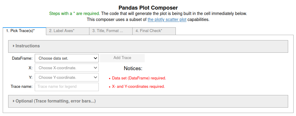
Figure 3: Image of the first tab in the four tab (4 step) Pandas Plot Composer. More information in the Pandas_GUI documentation.
It is best to do the tabs in order. The notices in red will try to warn you of errors or oversights. The "Instructions" accordian can be expanded to get more specific information about how to use each tab.
You can get more sophisticated control of your plot by editing the code produced by this GUI. See the Plotly FigureWidget Instructions and the example Jupyter notebooks referenced there for more information.
The GUI destroys itself once you complete step 4.
Analyzing data
Calculating a new column
Selecting "Calculate new column..." from the menu will a cell
immediately below the selected cell and launch the GUI to
lead you through creation of the code to calculate the new column. The code
is created immediately below the GUI. The first tab of the GUI looks like
figure 4. The command equivalent is newCalculatedColumn().
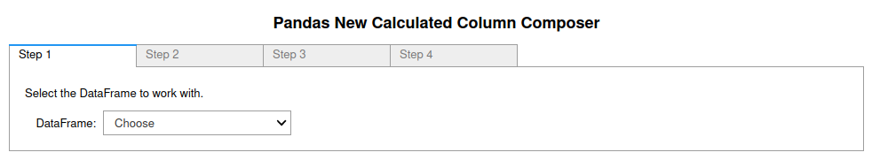
Figure 4: Image of the first tab in the four tab (4 step) Pandas New Calculated Column Composer. More information in the Pandas_GUI documentation.
Do the tabs in order. You can perform more complex manipulations than built into the GUI by editing the code generated by this GUI.
The GUI destroys itself once you complete step 4.
Fitting data
A GUI for defining simple fits (linear, polynomial, exponential decay, sine
and Gaussian) can be launched by selecting "Insert new fit after selected
cell" from the menu. This will create the GUI to lead you through selecting
and fitting the data. The code is created the immediately below the
GUI. The command equivalent is newFit().
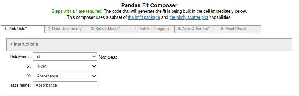
Figure 5: Image of the first tab in the Pandas Fit Composer. More information in the Pandas_GUI documentation.
Installation
Initial setup: On Raspberry Pi | On non-Pi Systems
Raspberry Pi Initial Setup
Unless you only want to run in Demo mode make sure you have one of the compatible interface boards installed. The current options are:
- Adafruit compliant ADS1115 boards (example, also available from other vendors);
- The π-Plates DAQC2 plate.
- If you wish to use different interfaces see the Development
Notes
and the
Boardssubpackage ofjupyterpidaqfor examples and information on how to define the code interface for a board.
OS specific: Ubuntu on Pi | Raspberrian on Pi | MacOS | Windows
Ubuntu on Pi
By default in Ubuntu 20.04 for Pis the gpio and spi groups do not exist. The i2c group does (not always).
- Make sure that the following packages are installed
rpi.gpio-common python3-pigpio python3-gpiozero python3-rpi.gpio. - You can avoid having to create a gpio group, by assigning users who need gpio access to the dialout group. Check that /dev/gpiomem is part of that group and that the dialout group has rw access. If not you will need to set it.
- Users also need to be members of the i2c group. If it does not exist create it and then make that the group for /dev/i2c-1 with group rw permissions. THIS MAY NOT BE NECESSARY.
- The spi group needs to be created (addgroup?).
- Additionally the spi group needs to be given rw access to the spi devices
at each boot. To do this create a one line rule in a file named
/etc/udev/rules.d/50-spidev.rulescontainingSUBSYSTEM=="spidev", GROUP="spi", MODE="0660". The file should have rw permission for root and read permission for everyone else. - Make sure you have pip installed for
python 3:
python3 -m pip --versionorpip3 --version. If you do not, install usingapt install python3-pip.
Raspberrian on Pi
(TBD)
Non-Pi based System Initial Setup
Make sure that Python >=3.6 is installed: python3 -v. If not follow
instructions at python.org. This software should run
on any computer capable of supporting the necessary version of Python.
Howevever, it will only run in demo mode if the computer does not support
one of the compatible A-to-D boards.
Generic Linux
- If your system hardware has GPIO pins and a GPIO interface board, you should try following the instructions for a Pi based system above. If you figure out how to make this work on other SBCs or systems with GPIO, please submit a pull request updating these instructions.
- If your system hardware does not support GPIO and one of the compatible interface boards, the software will run in demo mode.
NOTE: If a binary distribution (whl or wheel) is not available for your
platform, some of the required packages may need to be compiled. If you get
compilation errors when installing try getting the python header and
development files for your platform. To get them on most *nix platforms use the
command sudo apt install python3-dev.
MacOS
Currently, the LabQuest A-to-Ds are only working on intel based macs. When Vernier recompiles their interface communication library for the M1 series cpus this will change.
- Install the latest version of Python, by following the instructions on the Python website.
- Make sure a virtual environment tool such as
pipenvis installed. In a terminal window trypython -m pip install --user pipenv.
Windows
Note: LoggerPro software may need to be
installed because that provides the compiled .dll necessary to communicate
with the LabQuest interface. In theory will work without this.
- Install the latest version of Python, by following the instructions on the Python website. WARNING: Do Not use Windows automatic installation. It may work on a plain vanilla system with one user, but in multiuser systems it badly messes up the ability to use virtual environments.
- Make sure a virtual environment tool such as
pipenvis installed. In a terminal window trypython -m pip install --user pipenv. - You may have to set or add to your user
PATHenvironment variable. See the warnings generated during the installation. Then search for the latest instructions on how to setPATH.
Final Set Up
- If on Raspberry Pi type system, make sure the user you will be running the
software under is a member of the groups
dialout,spiand if it existsi2c. - It is recommended that you install JupyterPiDAQ in its own virtual environment. The instructions below do just that using the original author's favorite virtual environment tool pipenv.
Log into your chosen user account:
- Install pipenv:
pip3 install --user pipenv. You may need to add~/.local/binto yourPATHto makepipenvavailable in your command shell. More discussion: The Hitchhiker's Guide to Python. - Create a directory for the virtual environment you will be installing
into (example:
mkdir JupyterPiDAQ). - Navigate into the directory
cd JupyterPiDAQ. - Create the virtual environment and enter it
pipenv shell. To get out of the environment you can issue theexitcommand on the command line. - While still in the shell install the latest JupyterPiDAQ and all its
requirements
pip install -U JupyterPiDAQ. This can take a long time, especially on a Raspberry Pi. On a Pi 3B+ (minimum requirement) it will probably not run without at least 1 GB of swap. See: Build Jupyter on a Pi for a discussion of adding swap space on a Pi. - Still within the environment shell test
this by starting jupyter
jupyter notebook,jupyter laborjupyter nbclassic. Jupyter should launch in your browser.- Open a new notebook using the default (Python 3) kernel.
- In the first cell import all from DAQinstance.py:
from jupyterpidaq.DAQinstance import *. In classic notebook this cell should load the DAQmenu at the end of the Jupyter notebook menu/icon bar. In Notebook and Lab DAQ Commands menu should appear on launch of Jupyter. If you do not have an appropriate A-to-D board installed you will get a message and the software will default to demo mode, substituting a random number generator for the A-to-D.
- If you wish, you can make this environment available to an alternate Jupyter
install as a special kernel when you are the user.
- Make sure you are running in your virtual environment
pipenv shellin the directory for virtual environment will do that. - Issue the command to add this as a kernel to your personal space:
python -m ipykernel install --user --name=<name-you-want-for-kernel>. - More information is available in the Jupyter/IPython documentation. A simple tutorial from Nikolai Jankiev (_Parametric Thoughts_) can be found here.
- Make sure you are running in your virtual environment
Development Notes
Code Repository
Setting up Development Environment
Basic requirements: Python 3.6+, associated pip and a Jupyter notebook. See: python.org and Jupyter.org.
- If not installed, install pipenv:
pip3 install
--user pipenv
. You may need to add~/.local/binto yourPATHto makepipenvavailable in your command shell. More discussion: The Hitchhiker's Guide to Python. - Navigate to the directory where this package will be
or has been downloaded to. Use
pipenvto install an "editable" package inside the directory as described below:- Start a shell in the environment
pipenv shell. - Install using pip.
- If you downloaded the git repository named "JupyterPiDAQ"
and have used that directory to build your virtual
environment:
pip install -e ../JupyterPiDAQ/. - If you are downloading from PyPi
pip install -e JupyterPiDAQ - Either should install all the additional packages this package depends upon. On a Raspberry Pi this will take a long time. It probably will not run without at least 1 GB of swap. See: Build Jupyter on a Pi .
- If you downloaded the git repository named "JupyterPiDAQ"
and have used that directory to build your virtual
environment:
- Still within the environment shell test this by starting jupyter
jupyter nbclassicorjupyter lab. Jupyter should launch in your browser.- Open a new notebook using the default (Python 3) kernel.
- In the first cell import all from DAQinstance.py:
from jupyterpidaq.DAQinstance import *. When run this cell should load the DAQmenu at the end of the Jupyter notebook menu/icon bar. If you do not have an appropriate A-to-D board installed you will get a message and the software will default to demo mode, substituting a random number generator for the A-to-D. Because of the demo mode it is possible to run this on any computer, not just a Pi.
- Start a shell in the environment
- If you wish, you can make this environment available to an alternate Jupyter
install as a special kernel when you are the user.
- Make sure you are running in your virtual environment
pipenv shellin the directory for virtual environment will do that. - Issue the command to add this as a kernel to your personal space:
python -m ipykernel install --user --name=<name-you-want-for-kernel>. - More information is available in the Jupyter/Ipython documentation. A simple tutorial from Nikolai Jankiev (_Parametric Thoughts_) can be found here.
- Make sure you are running in your virtual environment
Adding New Sensor Code
- Copy an existing sensor class paste it into the end of sensors.py and rename it.
- Update/delete functions for each valid unit within the new class as necessary.
- Update the sensor name, vendor and available units in the
__init__function. - Add the new sensor classname to the list of available sensors
in
listSensorsat about line 120 of sensors.py. - Add the new sensor classname to
getsensorsof ADCsim.py, ADCsim_line.py and any board (e.g. DAQC2.py) with which the sensor can be used. Do not guess if a sensor works with a particular board. Test it!
Running Tests
- Install updated pytest in the virtual environment:
pipenv shell pip install -U pytest - Run tests ignoring the manual tests in the
dev_testingdirectory:python -m pytest --ignore='dev_testing'.
Building Documentation
- Install or update pdoc into the virtual environment
pip install -U pdoc. - Make edits to the
.mdfiles within the docs folder that are to be included in the first page (see__init__.pyof the jupyterpidaq package). - At the root level run
pdoc
--logo https://jupyterphysscilab.github.io/JupyterPiDAQ/JupyterPiDAQ-logo.svg --logo-link
https://jupyterphysscilab.github.io/JupyterPiDAQ/ --footer-text
"JupyterPiDAQ vX.X.X" -html -o docs jupyterpidaq
Unless you are on a Raspbery Pi this will throw an error aboutimport. Just ignore.
Building PyPi package
- Make sure to update the version number in setup.py first.
- Install updated setuptools and twine in the virtual environment:
pipenv shell pip install -U setuptools wheel twine - Build the distribution
python -m setup sdist bdist_wheel. - Test it on
test.pypi.org.- Upload it (you will need an account on test.pypi.org):
python -m twine upload --repository testpypi dist/*. - Create a new virtual environment and test install into it:
There are often install issues because sometimes only older versions of some of the required packages are available on test.pypi.org. If this is the only problem change the version to end inexit # to get out of the current environment cd <somewhere> mkdir <new virtual environment> cd <new directory> pipenv shell #creates the new environment and enters it. pip install -i https://test.pypi.org/..... # copy actual link from the # repository on test.pypi.rc0for release candidate and try it on the regular pypi.org as described below for releasing on PyPi. - After install test by running a jupyter notebook in the virtual environment.
- Upload it (you will need an account on test.pypi.org):
Releasing on PyPi
Proceed only if testing of the build is successful.
- Double check the version number in setup.py.
- Rebuild the release:
python -m setup sdist bdist_wheel. - Upload it:
python -m twine upload dist/* - Make sure it works by installing it in a clean virtual environment. This
is the same as on test.pypi.org except without
-i https://test.pypy.... If it does not work, pull the release.
Change Log
- 0.8.2 (July, 10, 2024)
- BUG FIX: Increased checking to avoid javascript errors in Jupyter Lab and Notebook 7+, while maintaining NBClassic capabilities.
- Added version of "DAQ Commands" menu that works in Jupyter Lab and Notebook 7+.
- Documentation updates and improvements.
- 0.8.1 (May 2, 2023)
- BUG FIX: Now always waits for all data to be transferred to plot before writing backup to a file.
- More rapid update of display when using LabQuests.
- Docs now recommend launching
jupyter nbclassicfor old notebook interface.
- 0.8.0 (Apr. 20, 2023)
- Replaced
NewRun()command withRun()command. This version works in Jupyter Lab and removes the need for theDisplayRun()command becauseRun()will load an already collected dataset or start a new one. - Now, when multiple traces are assigned to the same channel of a board the channel is only read one time. If the units are different the two traces will be displayed with different units.
- Can read data from Vernier LabQuest USB analog-to-digital interfaces. Potential data rate is 10 kHz, currently limited to 20 Hz.
- Runs in Jupyter Lab (no menus yet) and Notebook (menus still work).
- Updated requirements to include jupyterlab and labquest packages.
- Replaced
- 0.7.9 (Mar. 9 2023)
- Added
spidevpackage to requirements becausepi-platesrequires it. - More robust exception handling when searching for boards/A-to-Ds.
- Added
- 0.7.8
- Updated text for insertion into cells to make better use of escaping updates in JPSLUtils >=0.7.0.
- Removed some unnecessary print statements.
- 0.7.7
- Updated requirements for upstream security fixes.
- Conversion to pandas dataframe now works when trace 0 is not collected.
- DAQ menu no longer created in trusted notebooks if the data acquisition tools have not been initialized since the notebook was opened.
- Reworked the data collection so that opening an old notebook without running anything will not have any leftover inoperable or undefined widgets.
- Reordered the live trace display to match the order of the names at right.
- Runs now saved to a human readable html file that includes the run conditions.
- As long as this html file is in the same directory as the notebook, the run display can be recreated by running its cell after accidentally clearing the cell output.
- The cell displaying the results of a run is now protected against deletion and editing.
- 0.7.6
- Converted to fancy menus (could make hierarchical).
- 0.7.5
- Added fitting to DAQ command menu.
- Documentation Enhancements: github.io website; first pass as API docs; reorganized documentation; MyBinder link now forces launch in classic notebook; added plans for adapter board to connect Vernier Sensors.
- 0.7.4.1
- Improved layout of data collection.
- Better widget cleanup.
- Readme fixes.
- 0.7.3 Pip install reliability fixes.
- 0.7.2 Suppress Javascript error when not in JLab.
- 0.7.1
- Include Heat Capacity Lab example.
- Make menu show up in JLab (still not functional).
- Remove matplotlib baggage.
- 0.7.0
- Switched to plotly widget for plotting.
- Added Vernier pressure sensor calibrations (old and new).
- Jupyter widgets based new calculated column GUI.
- Jupyter widgets based new plot GUI.
- Default to providing only one time for channels collected nearly simultaneously.
- As reported values are averages, switched to reporting the estimated standard deviation of the average rather than the deviation of all the readings used to create the average.
- 0.6.0
- Initial release.
- Live data collection.
- Recognized sensors: ADS1115 boards (voltage, built-in thermistor, Vernier SS temperature probe), DAQC2 boards (voltage,Vernier SS temperature probe, Vernier standard pH probe, Vernier flat pH probe).
Three Channel Adapter Board for Vernier Sensors
Board plans

Etching the board
Clean Cu cladding to be etched by wet sanding with 1500 grit or finer. Draw traces with a black sharpie “industrial super permanent ink” version works best. Allow to dry completely (no odor). Can be speeded up using a heat gun.
Etchant recipe:
3 M HCl
CuCl2 to make medium emerald green solution (can also be made by dissolving Cu after adding hydrogen peroxide)
Using test piece add 30% H2O2 dropwise to get gentle bubbling and complete removal in 3 – 5 min (longer gives poorly defined edges).