Fits to an exponential relaxation from an initial to a final value using fit_pandas_GUI()
You can try this notebook live by lauching it in Binder.This can take a while to launch, be patient.
![]() .
.
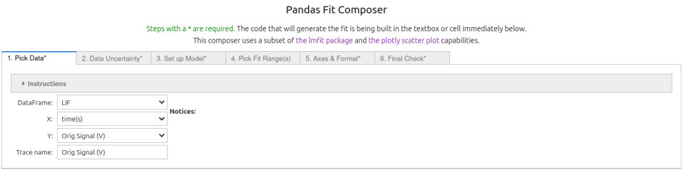
Real Laser Induced Fluoresence (LIF) data from quinine sulfate in sulfuric acid measured at a wavelenth of 480 nm are analyzed below.
First we import the data set into a pandas dataframe, then invert it and add an offset (this recovers the orginal raw form of the data):
import pandas as pd
LIF = pd.read_csv('DataSets/LIF.csv')
LIF['Orig Signal (V)'] = -LIF['Signal (V)'] - 0.04
To facilitate plotting and analysis we will import the pandas_GUI package:
from pandas_GUI import *
Let's make a quick plot to look at the raw data, using the plot_pandas_GUI()
This was done by running the command plot_pandas_GUI() in an empty code cell. The code and plot created are shown in the cell after this one. To learn more about using the plot_pandas_GUI() start with the
step-by-step example.
# CODE BLOCK generated using plot_pandas_GUI().
# See https://jupyterphysscilab.github.io/jupyter_Pandas_GUI.
from plotly import graph_objects as go
Figure_1 = go.FigureWidget(layout_template="simple_white")
# Trace declaration(s) and trace formatting
scat = go.Scatter(x = LIF['time(s)'], y = LIF['Orig Signal (V)'],
mode = 'lines', name = 'Orig Signal (V)',)
Figure_1.add_trace(scat)
# Axes labels
Figure_1.update_xaxes(title= 'time (s)')
Figure_1.update_yaxes(title= 'raw signal (V)')
# Plot formatting
Figure_1.update_layout(title = 'Figure_1', template = 'simple_white', autosize=True)
display(Figure_1)
Figure 1: A plot of the raw signal. Notice that it decays towards a value near -0.04 V from less than -0.07 V.
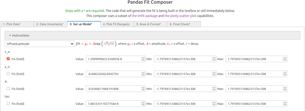
3. On the third tab
the 'OffsetExp' model was chosen from the pop-up menu. In this case the default initial guesses identified the peak where the exponential starts (minimum). Generally the $x_o$ value should be set manually and fixed to get good fits. Because the default guess for $x_o$ is so good it was kept and the "fix" box was checked. All the other parameters were allowed to vary.
4. On the fourth tab
the range of data was selected by clicking on the first and last point in the range to fit.

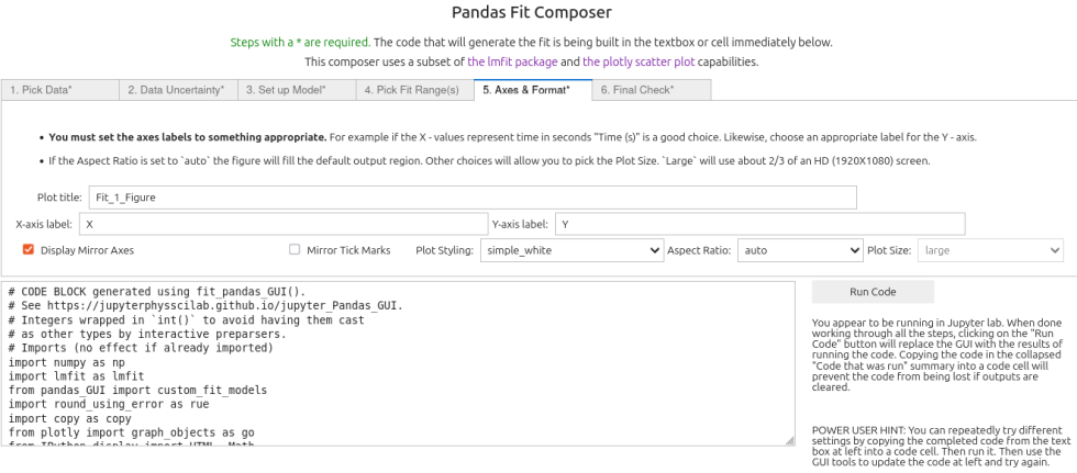
6. On the last (sixth) tab
the final checks were done and then the 'Run Code' button was clicked, replacing the GUI with the results. It is best to copy the collapsed code into a new cell to save the ability to recreate the graph if the widget cannot be recreated.
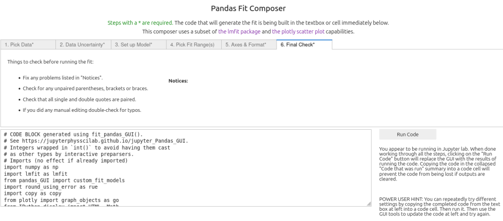
After dealing with any errors noted the user can then click on the "Run Code" button and get a display of the results.
HOWEVER, Jupyter saving of widget states varies in reliability as things are updated. Thus it is best to copy the code into a new cell, so that the code that generates the fit and plot is saved and can be rerun to generate the results and plot. This can be done by copying the code in the textbox without clicking "Run Code" or by expanding the "Code that was run" block and copying from that after using the "Run Code" button. An image of the result from clicking "Run Code" is below.
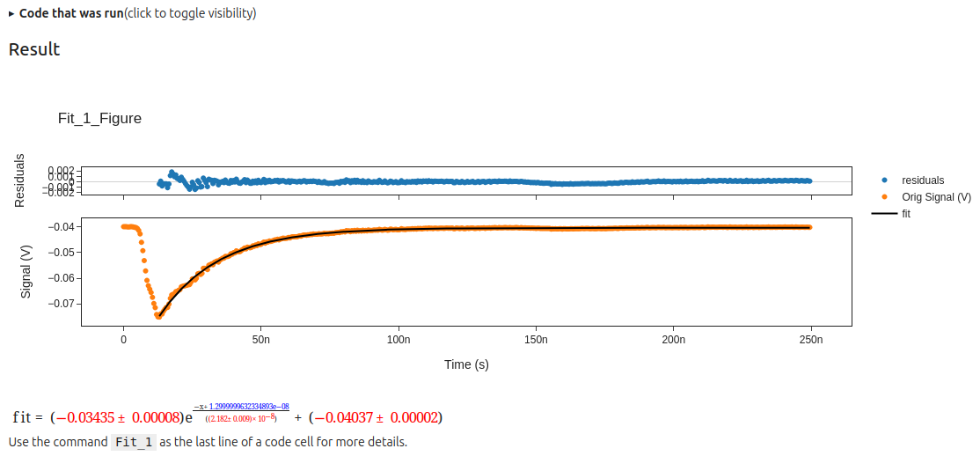
The code below was copied from the "Code that was run" expanding tab above. Running it recreates the fit above. Depending on the current status of widget state saving, the live interactive plot may or may not show in an active notebook. Rerunning the notebook from the beginning will regenerate the live interactive plot.
# CODE BLOCK generated using fit_pandas_GUI().
# See https://jupyterphysscilab.github.io/jupyter_Pandas_GUI.
# Integers wrapped in `int()` to avoid having them cast
# as other types by interactive preparsers.
# Imports (no effect if already imported)
import numpy as np
import lmfit as lmfit
from pandas_GUI import custom_fit_models
import round_using_error as rue
import copy as copy
from plotly import graph_objects as go
from IPython.display import HTML, Math
# Define data and trace name
Xvals = LIF["time(s)"]
Yvals = LIF["Orig Signal (V)"]
tracename = "Orig Signal (V)"
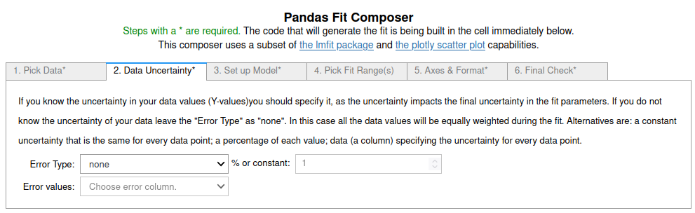
# Define error (uncertainty)
Yerr = LIF["Orig Signal (V)"]*0.0 + 1.0
# Define the fit model, initial guesses, and constraints
fitmod = custom_fit_models.OffsetExpModel()
fitmod.set_param_hint("x_o", vary = False, value = 1.2999999632334893e-08)
fitmod.set_param_hint("y_o", vary = True, value = -0.0402265624942765)
fitmod.set_param_hint("A", vary = True, value = -0.0348671866191808)
fitmod.set_param_hint("tau", vary = True, value = 7.88333311037744e-08)
# Define fit ranges
Yfiterr = copy.deepcopy(Yerr) # ranges not to fit = np.inf
Xfitdata = copy.deepcopy(Xvals) # ranges where fit not displayed = np.nan
Yfiterr[int(0):int(26)] = np.inf
Xfitdata[int(0):int(26)] = np.nan
Yfiterr[int(500):int(500)] = np.inf
Xfitdata[int(500):int(500)] = np.nan
# Do fit
Fit_1 = fitmod.fit(Yvals, x=Xvals, weights = 1/Yfiterr, scale_covar = True, nan_policy = "omit")
# Calculate residuals (data - fit) because lmfit
# does not calculate for all points under all conditions
resid = []
# explicit int(0) below avoids collisions with some preparsers.
for i in range(int(0),len(Fit_1.data)):
resid.append(Fit_1.data[i]-Fit_1.best_fit[i])
# Delete residuals in ranges not fit
# and fit values that are not displayed.
for i in range(len(resid)):
if np.isnan(Xfitdata[i]):
resid[i] = None
Fit_1.best_fit[i] = None
# Plot Results
# explicit int(..) below avoids collisions with some preparsers.
Fit_1_Figure = go.FigureWidget(layout_template="simple_white")
Fit_1_Figure.update_layout(title = "Fit_1_Figure",autosize=True)
Fit_1_Figure.set_subplots(rows=int(2), cols=int(1), row_heights=[0.2,0.8], shared_xaxes=True)
scat = go.Scatter(y=resid,x=Xfitdata, mode="markers",name = "residuals")
Fit_1_Figure.update_yaxes(title = "Residuals", row=int(1), col=int(1), zeroline=True, zerolinecolor = "lightgrey", mirror = True)
Fit_1_Figure.update_xaxes(row=int(1), col=int(1), mirror = True)
Fit_1_Figure.add_trace(scat,col=int(1),row=int(1))
scat = go.Scatter(x=Xvals, y=Yvals, mode="markers", name=tracename)
Fit_1_Figure.add_trace(scat, col=int(1), row=int(2))
Fit_1_Figure.update_yaxes(title = "Signal (V)", row=int(2), col=int(1), mirror = True)
Fit_1_Figure.update_xaxes(title = "Time (s)", row=int(2), col=int(1), mirror = True)
scat = go.Scatter(y=Fit_1.best_fit,x=Xfitdata, mode="lines", name="fit", line_color = "black", line_dash="solid")
Fit_1_Figure.add_trace(scat,col=int(1),row=int(2))
display(Fit_1_Figure)
# Display best fit equation
rawlatex = r'A e^{\frac{- x + x_{o}}{\tau}} + y_{o}' # via sympy
from sympy import sympify, latex
for k in Fit_1.params.keys():
if Fit_1.params[k].vary:
paramstr = r'({\color{red}{'+rue.latex_rndwitherr(Fit_1.params[k].value,
Fit_1.params[k].stderr,
errdig=int(1),
lowmag=-int(3))+'}})'
else:
paramstr = r'{\color{blue}{'+str(Fit_1.params[k].value,
)+'}}'
rawlatex = rawlatex.replace(latex(sympify(k)),paramstr)
fitstr = r'$$fit = '+rawlatex+'$$'
captionstr = r'<p>Use the command <code>Fit_1</code> as the last line of a code cell for more details.</p>'
display(Math(fitstr))
display(HTML(captionstr))
Use the command Fit_1 as the last line of a code cell for more details.