Exponential Fits using fit_pandas_GUI()

You can try this notebook live by lauching it in Binder.This can take a while to launch, be patient. .

Two Laser Induced Fluoresence (LIF) signals from quinine sulfate in sulfuric acid measured at a wavelenth of 480 nm are analyzed below.

First we import the data sets into pandas dataframes:

import pandas as pd
LIF = pd.read_csv('DataSets/LIF.csv')
LIF2 = pd.read_csv('DataSets/LIF2.csv')

To facilitate plotting and analysis we will import the pandas_GUI package:

from pandas_GUI import *

Let's make a quick plot to look at the raw data, using the plot_pandas_GUI()

This was done by running the command plot_pandas_GUI() in an empty code cell. The code and plot created are shown in the cell after this one. To learn more about using the plot_pandas_GUI() start with the step-by-step example.

# CODE BLOCK generated using plot_pandas_GUI(). See https://github.com/JupyterPhysSciLab/jupyter_Pandas_GUI.
from plotly import graph_objects as go
Figure_1 = go.FigureWidget(layout_template="simple_white")
scat = go.Scatter(x = LIF['time(s)'], y = LIF['Signal (V)'],
        mode = 'lines', name = 'LIF1',)
Figure_1.add_trace(scat)
scat = go.Scatter(x = LIF2['time(s)'], y = LIF2['Signal (V)'],
        mode = 'lines', name = 'LIF2',)
Figure_1.add_trace(scat)
Figure_1.update_xaxes(title= 'Time (s)', mirror = True)
Figure_1.update_yaxes(title= 'Signal (V)', mirror = True)
Figure_1.update_layout(title = 'Figure_1', template = 'simple_white')
Figure_1.show(config = {'toImageButtonOptions': {'format': 'svg'}})

Figure 1: A plot of the two signals. Notice that LIF2 exhibits a step at the base of the decay (17 to 30 ns). This is due to a small secondary pulse of the excitation laser, after the initial signal has started to decay. The LIF1 data is impacted much less by the small secondary pulse.

Example 1: Fitting the slower decay (LIF1) using the fit_pandas_GUI()

The fit was done by running the command fit_pandas_GUI() in an empty code cell.

1. On the first tab

the data set, which columns contained the X- and Y-data and a name for the trace were chosen.

2. On the second tab

the the default 'none' value was kept for uncertainties.

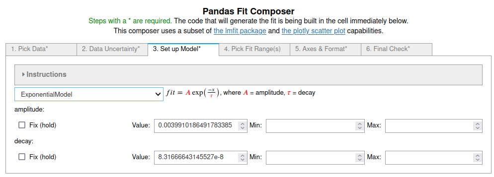
3. On the third tab

the 'Exponential' model was chosen from the pop-up menu. The default initial guesses were used.

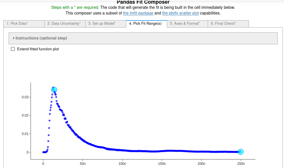
4. On the fourth tab

the range of data was selected by clicking on the first and last point in the range to fit.

5. On the fifth tab

the axes titles were entered and the 'mirror axes' box checked.

6. On the last (sixth) tab

the final checks were done and then the 'Do Fit' button was clicked, closing the GUI and running the code in the cell below to perform the fit and display the results.

# CODE BLOCK generated using fit_pandas_GUI().
# See https://jupyterphysscilab.github.io/jupyter_Pandas_GUI.
# Integers wrapped in `int()` to avoid having them cast 
# as other types by interactive preparsers. 
# Imports (no effect if already imported)
import numpy as np
import lmfit as lmfit
import round_using_error as rue
import copy as copy
from plotly import graph_objects as go
from IPython.display import HTML, Math

# Define data and trace name
Xvals = LIF["time(s)"]
Yvals = LIF["Signal (V)"]
tracename = "LIF1"

# Define error (uncertainty)
Yerr = LIF["Signal (V)"]*0.0 + 1.0

# Define the fit model, initial guesses, and constraints
fitmod = lmfit.models.ExponentialModel()
fitmod.set_param_hint("amplitude", vary = True, value = 0.0039910186491783385)
fitmod.set_param_hint("decay", vary = True, value = 8.31666643145527e-08)

# Define fit ranges
Yfiterr = copy.deepcopy(Yerr) # ranges not to fit = np.inf
Xfitdata = copy.deepcopy(Xvals) # ranges where fit not displayed = np.nan
Yfiterr[int(0):int(28)] = np.inf
Xfitdata[int(0):int(28)] = np.nan
Yfiterr[int(500):int(500)] = np.inf
Xfitdata[int(500):int(500)] = np.nan

# Do fit
Fit_1 = fitmod.fit(Yvals, x=Xvals, weights = 1/Yfiterr, scale_covar = True, nan_policy = "omit")

# Calculate residuals (data - fit) because lmfit
#  does not calculate for all points under all conditions
resid = []
# explicit int(0) below avoids collisions with some preparsers.
for i in range(int(0),len(Fit_1.data)):
    resid.append(Fit_1.data[i]-Fit_1.best_fit[i])

# Delete residuals in ranges not fit
# and fit values that are not displayed.
for i in range(len(resid)):
    if np.isnan(Xfitdata[i]):
        resid[i] = None
        Fit_1.best_fit[i] = None

# Plot Results
# explicit int(..) below avoids collisions with some preparsers.
Fit_1_Figure = go.FigureWidget(layout_template="simple_white")
Fit_1_Figure.update_layout(title = "Fit_1_Figure",autosize=True)
Fit_1_Figure.set_subplots(rows=int(2), cols=int(1), row_heights=[0.2,0.8], shared_xaxes=True)
scat = go.Scatter(y=resid,x=Xfitdata, mode="markers",name = "residuals")
Fit_1_Figure.update_yaxes(title = "Residuals", row=int(1), col=int(1), zeroline=True, zerolinecolor = "lightgrey", mirror = True)
Fit_1_Figure.update_xaxes(row=int(1), col=int(1), mirror = True)
Fit_1_Figure.add_trace(scat,col=int(1),row=int(1))
scat = go.Scatter(x=Xvals, y=Yvals, mode="markers", name=tracename)
Fit_1_Figure.add_trace(scat, col=int(1), row=int(2))
Fit_1_Figure.update_yaxes(title = "Signal (V)", row=int(2), col=int(1), mirror = True)
Fit_1_Figure.update_xaxes(title = "Time (s)", row=int(2), col=int(1), mirror = True)
scat = go.Scatter(y=Fit_1.best_fit,x=Xfitdata, mode="lines", name="fit", line_color = "black", line_dash="solid")
Fit_1_Figure.add_trace(scat,col=int(1),row=int(2))
Fit_1_Figure.show(config = {'toImageButtonOptions': {'format': 'svg'}})

# Display best fit equation
ampstr = ''
decaystr = ''
for k in Fit_1.params.keys():
    if Fit_1.params[k].vary:
        paramstr = r'({\color{red}{'+rue.latex_rndwitherr(Fit_1.params[k].value,
                                 Fit_1.params[k].stderr,
                                 errdig=int(1),
                                 lowmag=-int(3))+'}})'
    else:
        paramstr = r'{\color{blue}{'+str(Fit_1.params[k].value, 
                                       )+'}}'
    if k == 'amplitude':
        ampstr = paramstr
    if k == 'decay':
        decaystr = paramstr
fitstr = r'$$fit = '+ampstr+r'\exp \left( \frac{-x}{'+decaystr+r'}\right)$$'
captionstr = r'<p>Use the command <code>Fit_1</code> as the last line of a code cell for more details.</p>'
display(Math(fitstr))
display(HTML(captionstr))

$\displaystyle fit = ({\color{red}{0.0605\pm0.0004}})\exp \left( \frac{-x}{({\color{red}{(2.29\pm0.01)\times 10^{-8}}})}\right)$

Use the command Fit_1 as the last line of a code cell for more details.

Fit 1: In this case the whole decay from the peak to the end of the data set was fit. Notice that the fit equation, including estimated errors of the fit parameters, is displayed as a typeset equation. The residuals suggest there is significant noise on the early part of the signal, possibly because the laser pulse did not shut off completely. There is also a signal between 150 and 200 ns, that appears to be a reflection of the signal in the cabling due to a slight mismatch of the termination impedence.

Example 2: Fitting the faster decay

The code and fit below were generated the same way as example 1, but using the faster decaying LIF2 data set.

# CODE BLOCK generated using fit_pandas_GUI().
# See https://jupyterphysscilab.github.io/jupyter_Pandas_GUI.
# Integers wrapped in `int()` to avoid having them cast 
# as other types by interactive preparsers. 
# Imports (no effect if already imported)
import numpy as np
import lmfit as lmfit
import round_using_error as rue
import copy as copy
from plotly import graph_objects as go
from IPython.display import HTML, Math

# Define data and trace name
Xvals = LIF2["time(s)"]
Yvals = LIF2["Signal (V)"]
tracename = "LIF2"

# Define error (uncertainty)
Yerr = LIF2["Signal (V)"]*0.0 + 1.0

# Define the fit model, initial guesses, and constraints
fitmod = lmfit.models.ExponentialModel()
fitmod.set_param_hint("amplitude", vary = True, value = 0.003681165532005888)
fitmod.set_param_hint("decay", vary = True, value = 4.158333215727635e-08)

# Define fit ranges
Yfiterr = copy.deepcopy(Yerr) # ranges not to fit = np.inf
Xfitdata = copy.deepcopy(Xvals) # ranges where fit not displayed = np.nan
Yfiterr[int(0):int(50)] = np.inf
Xfitdata[int(0):int(50)] = np.nan
Yfiterr[int(500):int(500)] = np.inf
Xfitdata[int(500):int(500)] = np.nan

# Do fit
Fit_2 = fitmod.fit(Yvals, x=Xvals, weights = 1/Yfiterr, scale_covar = True, nan_policy = "omit")

# Calculate residuals (data - fit) because lmfit
#  does not calculate for all points under all conditions
resid = []
# explicit int(0) below avoids collisions with some preparsers.
for i in range(int(0),len(Fit_2.data)):
    resid.append(Fit_2.data[i]-Fit_2.best_fit[i])

# Delete residuals in ranges not fit
# and fit values that are not displayed.
for i in range(len(resid)):
    if np.isnan(Xfitdata[i]):
        resid[i] = None
        Fit_2.best_fit[i] = None

# Plot Results
# explicit int(..) below avoids collisions with some preparsers.
Fit_2_Figure = go.FigureWidget(layout_template="simple_white")
Fit_2_Figure.update_layout(title = "Fit_2_Figure",autosize=True)
Fit_2_Figure.set_subplots(rows=int(2), cols=int(1), row_heights=[0.2,0.8], shared_xaxes=True)
scat = go.Scatter(y=resid,x=Xfitdata, mode="markers",name = "residuals")
Fit_2_Figure.update_yaxes(title = "Residuals", row=int(1), col=int(1), zeroline=True, zerolinecolor = "lightgrey", mirror = True)
Fit_2_Figure.update_xaxes(row=int(1), col=int(1), mirror = True)
Fit_2_Figure.add_trace(scat,col=int(1),row=int(1))
scat = go.Scatter(x=Xvals, y=Yvals, mode="markers", name=tracename)
Fit_2_Figure.add_trace(scat, col=int(1), row=int(2))
Fit_2_Figure.update_yaxes(title = "Signal (V)", row=int(2), col=int(1), mirror = True)
Fit_2_Figure.update_xaxes(title = "Time (s)", row=int(2), col=int(1), mirror = True)
scat = go.Scatter(y=Fit_2.best_fit,x=Xfitdata, mode="lines", name="fit", line_color = "black", line_dash="solid")
Fit_2_Figure.add_trace(scat,col=int(1),row=int(2))
Fit_2_Figure.show(config = {'toImageButtonOptions': {'format': 'svg'}})

# Display best fit equation
ampstr = ''
decaystr = ''
for k in Fit_2.params.keys():
    if Fit_2.params[k].vary:
        paramstr = r'({\color{red}{'+rue.latex_rndwitherr(Fit_2.params[k].value,
                                 Fit_2.params[k].stderr,
                                 errdig=int(1),
                                 lowmag=-int(3))+'}})'
    else:
        paramstr = r'{\color{blue}{'+str(Fit_2.params[k].value, 
                                       )+'}}'
    if k == 'amplitude':
        ampstr = paramstr
    if k == 'decay':
        decaystr = paramstr
fitstr = r'$$fit = '+ampstr+r'\exp \left( \frac{-x}{'+decaystr+r'}\right)$$'
captionstr = r'<p>Use the command <code>Fit_2</code> as the last line of a code cell for more details.</p>'
display(Math(fitstr))
display(HTML(captionstr))

$\displaystyle fit = ({\color{red}{0.65\pm0.03}})\exp \left( \frac{-x}{({\color{red}{(4.61\pm0.06)\times 10^{-9}}})}\right)$

Use the command Fit_2 as the last line of a code cell for more details.

Fit 2: Again the fit region is from the beginning of the decay to the end of the data set. Notice that the fit is skewed by the blip at the base of the primary decay caused by the secondary pulse of the laser.

Example 3: Fitting the faster decay, but ignoring the blip from the secondary laser pulse

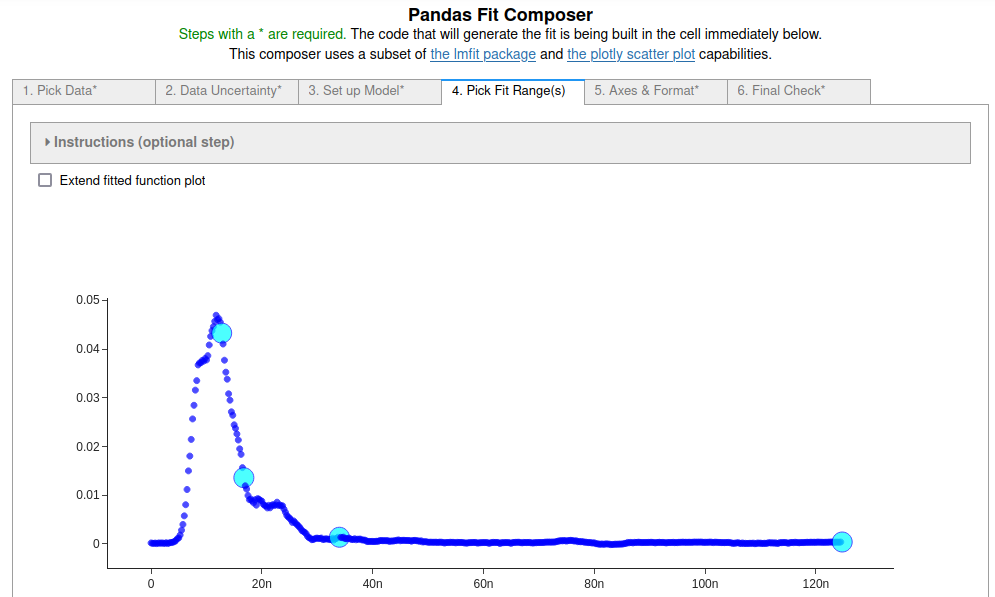
The blip disrupts the data pretty badly, so trying to fit around it probably does not yield particularly good results, but this example used the data to illustrate how to fit to discontiguous regions of a data set.

Everything was done exactly the same as in the first two examples except that two fit ranges, before the blip and after the blip, were defined on tab 4 by selecting two additional points as shown in the figure below. Consecutive pairs of points starting from the lowest point index define the fit ranges.

# CODE BLOCK generated using fit_pandas_GUI().
# See https://jupyterphysscilab.github.io/jupyter_Pandas_GUI.
# Integers wrapped in `int()` to avoid having them cast 
# as other types by interactive preparsers. 
# Imports (no effect if already imported)
import numpy as np
import lmfit as lmfit
import round_using_error as rue
import copy as copy
from plotly import graph_objects as go
from IPython.display import HTML, Math

# Define data and trace name
Xvals = LIF2["time(s)"]
Yvals = LIF2["Signal (V)"]
tracename = "LIF2"

# Define error (uncertainty)
Yerr = LIF2["Signal (V)"]*0.0 + 1.0

# Define the fit model, initial guesses, and constraints
fitmod = lmfit.models.ExponentialModel()
fitmod.set_param_hint("amplitude", vary = True, value = 0.003681165532005888)
fitmod.set_param_hint("decay", vary = True, value = 4.158333215727635e-08)

# Define fit ranges
Yfiterr = copy.deepcopy(Yerr) # ranges not to fit = np.inf
Xfitdata = copy.deepcopy(Xvals) # ranges where fit not displayed = np.nan
Yfiterr[int(0):int(51)] = np.inf
Xfitdata[int(0):int(51)] = np.nan
Yfiterr[int(69):int(157)] = np.inf
Xfitdata[int(69):int(157)] = np.nan
Yfiterr[int(500):int(500)] = np.inf
Xfitdata[int(500):int(500)] = np.nan

# Do fit
Fit_3 = fitmod.fit(Yvals, x=Xvals, weights = 1/Yfiterr, scale_covar = True, nan_policy = "omit")

# Calculate residuals (data - fit) because lmfit
#  does not calculate for all points under all conditions
resid = []
# explicit int(0) below avoids collisions with some preparsers.
for i in range(int(0),len(Fit_3.data)):
    resid.append(Fit_3.data[i]-Fit_3.best_fit[i])

# Delete residuals in ranges not fit
# and fit values that are not displayed.
for i in range(len(resid)):
    if np.isnan(Xfitdata[i]):
        resid[i] = None
        Fit_3.best_fit[i] = None

# Plot Results
# explicit int(..) below avoids collisions with some preparsers.
Fit_3_Figure = go.FigureWidget(layout_template="simple_white")
Fit_3_Figure.update_layout(title = "Fit_3_Figure",autosize=True)
Fit_3_Figure.set_subplots(rows=int(2), cols=int(1), row_heights=[0.2,0.8], shared_xaxes=True)
scat = go.Scatter(y=resid,x=Xfitdata, mode="markers",name = "residuals")
Fit_3_Figure.update_yaxes(title = "Residuals", row=int(1), col=int(1), zeroline=True, zerolinecolor = "lightgrey", mirror = True)
Fit_3_Figure.update_xaxes(row=int(1), col=int(1), mirror = True)
Fit_3_Figure.add_trace(scat,col=int(1),row=int(1))
scat = go.Scatter(x=Xvals, y=Yvals, mode="markers", name=tracename)
Fit_3_Figure.add_trace(scat, col=int(1), row=int(2))
Fit_3_Figure.update_yaxes(title = "Signal (V)", row=int(2), col=int(1), mirror = True)
Fit_3_Figure.update_xaxes(title = "Time (s)", row=int(2), col=int(1), mirror = True)
scat = go.Scatter(y=Fit_3.best_fit,x=Xfitdata, mode="lines", name="fit", line_color = "black", line_dash="solid")
Fit_3_Figure.add_trace(scat,col=int(1),row=int(2))
Fit_3_Figure.show(config = {'toImageButtonOptions': {'format': 'svg'}})

# Display best fit equation
ampstr = ''
decaystr = ''
for k in Fit_3.params.keys():
    if Fit_3.params[k].vary:
        paramstr = r'({\color{red}{'+rue.latex_rndwitherr(Fit_3.params[k].value,
                                 Fit_3.params[k].stderr,
                                 errdig=int(1),
                                 lowmag=-int(3))+'}})'
    else:
        paramstr = r'{\color{blue}{'+str(Fit_3.params[k].value, 
                                       )+'}}'
    if k == 'amplitude':
        ampstr = paramstr
    if k == 'decay':
        decaystr = paramstr
fitstr = r'$$fit = '+ampstr+r'\exp \left( \frac{-x}{'+decaystr+r'}\right)$$'
captionstr = r'<p>Use the command <code>Fit_3</code> as the last line of a code cell for more details.</p>'
display(Math(fitstr))
display(HTML(captionstr))

$\displaystyle fit = ({\color{red}{1.19\pm0.04}})\exp \left( \frac{-x}{({\color{red}{(3.86\pm0.04)\times 10^{-9}}})}\right)$

Use the command Fit_3 as the last line of a code cell for more details.

Fit 3: A fit ignoring some of the region containing the blip. You can see that the fit to the initial part of the decay is better, but not perfect. Ignoring the blip is not adequate to account for the multiple pulses from the laser.

# CODE BLOCK generated using fit_pandas_GUI().
# See https://jupyterphysscilab.github.io/jupyter_Pandas_GUI.
# Integers wrapped in `int()` to avoid having them cast 
# as other types by interactive preparsers. 
# Imports (no effect if already imported)
import numpy as np
import lmfit as lmfit
import round_using_error as rue
import copy as copy
from plotly import graph_objects as go
from IPython.display import HTML, Math

# Define data and trace name
Xvals = LIF2["time(s)"]
Yvals = LIF2["Signal (V)"]
tracename = "LIF2"

# Define error (uncertainty)
Yerr = LIF2["Signal (V)"]*0.0 + 1.0

# Define the fit model, initial guesses, and constraints
fitmod = lmfit.models.ExponentialModel()
fitmod.set_param_hint("amplitude", vary = True, value = 0.003681165532005888)
fitmod.set_param_hint("decay", vary = True, value = 4.158333215727635e-08)

# Define fit ranges
Yfiterr = copy.deepcopy(Yerr) # ranges not to fit = np.inf
Xfitdata = copy.deepcopy(Xvals) # ranges where fit not displayed = np.nan
Yfiterr[int(0):int(51)] = np.inf
Xfitdata[int(0):int(51)] = np.nan
Yfiterr[int(69):int(157)] = np.inf
Xfitdata[int(69):int(157)] = np.nan
Yfiterr[int(500):int(500)] = np.inf
Xfitdata[int(500):int(500)] = np.nan

# Do fit
Fit_4 = fitmod.fit(Yvals, x=Xvals, weights = 1/Yfiterr, scale_covar = True, nan_policy = "omit")

# Calculate residuals (data - fit) because lmfit
#  does not calculate for all points under all conditions
resid = []
# explicit int(0) below avoids collisions with some preparsers.
for i in range(int(0),len(Fit_4.data)):
    resid.append(Fit_4.data[i]-Fit_4.best_fit[i])

# Plot Results
# explicit int(..) below avoids collisions with some preparsers.
Fit_4_Figure = go.FigureWidget(layout_template="simple_white")
Fit_4_Figure.update_layout(title = "Fit_4_Figure",autosize=True)
Fit_4_Figure.set_subplots(rows=int(2), cols=int(1), row_heights=[0.2,0.8], shared_xaxes=True)
scat = go.Scatter(y=resid,x=Xvals, mode="markers",name = "residuals")
Fit_4_Figure.update_yaxes(title = "Residuals", row=int(1), col=int(1), zeroline=True, zerolinecolor = "lightgrey", mirror = True)
Fit_4_Figure.update_xaxes(row=int(1), col=int(1), mirror = True)
Fit_4_Figure.add_trace(scat,col=int(1),row=int(1))
scat = go.Scatter(x=Xvals, y=Yvals, mode="markers", name=tracename)
Fit_4_Figure.add_trace(scat, col=int(1), row=int(2))
Fit_4_Figure.update_yaxes(title = "Signal (V)", row=int(2), col=int(1), mirror = True)
Fit_4_Figure.update_xaxes(title = "Time (s)", row=int(2), col=int(1), mirror = True)
scat = go.Scatter(y=Fit_4.best_fit, x=Xvals, mode="lines", line_color = "black", name="extrapolated",line_dash="dash")
Fit_4_Figure.add_trace(scat, col=int(1), row=int(2))
scat = go.Scatter(y=Fit_4.best_fit,x=Xfitdata, mode="lines", name="fit", line_color = "black", line_dash="solid")
Fit_4_Figure.add_trace(scat,col=int(1),row=int(2))
Fit_4_Figure.show(config = {'toImageButtonOptions': {'format': 'svg'}})

# Display best fit equation
ampstr = ''
decaystr = ''
for k in Fit_4.params.keys():
    if Fit_4.params[k].vary:
        paramstr = r'({\color{red}{'+rue.latex_rndwitherr(Fit_4.params[k].value,
                                 Fit_4.params[k].stderr,
                                 errdig=int(1),
                                 lowmag=-int(3))+'}})'
    else:
        paramstr = r'{\color{blue}{'+str(Fit_4.params[k].value, 
                                       )+'}}'
    if k == 'amplitude':
        ampstr = paramstr
    if k == 'decay':
        decaystr = paramstr
fitstr = r'$$fit = '+ampstr+r'\exp \left( \frac{-x}{'+decaystr+r'}\right)$$'
captionstr = r'<p>Use the command <code>Fit_4</code> as the last line of a code cell for more details.</p>'
display(Math(fitstr))
display(HTML(captionstr))

$\displaystyle fit = ({\color{red}{1.19\pm0.04}})\exp \left( \frac{-x}{({\color{red}{(3.86\pm0.04)\times 10^{-9}}})}\right)$

Use the command Fit_4 as the last line of a code cell for more details.

Fit 4: The same fit as Fit 3, but checking the 'Extend Fit' box. The dashed fit line indicates regions that were not fit. The fit and residuals are show for the whole range of the data set. If you are in a live notebook and zoom in you can see that the fit is the same as before. Additional zooming of the residuals is necessary to see details of them.